

Regression Trees

““A peacefulness follows any decision, even the wrong one.””
Objectives:
Gain an understanding of how regression trees are cultivated and pruned;
Programmatically create a regression tree using DecisionTree Regressor of sklearn;
Understand the mathematical function behind regression tree growing;
Learn about tree pruning in sklearn:
tune max_depth parameter with cross validation in for loop;
tune max_depth parameter with GridSearchCV;
Visualize a regression tree; and
Understand regression tree structures.
Overview:
Tree-based methods are predictive models that involve segmenting the feature space into several sub-regions. Since the divided feature space can be visualized as a tree, the approaches are often referred to as tree-based methods.
Tree-based models are relatively easy to explain and can be used for regression (e.g. when the dependent variable is continuous) and for classification (e.g. when the dependent variable is a class variable). Decision or regression trees are usually less accurate than other machine learning approaches like bagging, random forests and boosting, which cultivate several trees, which are then combined during prediction. As a result of the increased complexity, for regression (e.g. when the dependent variable is continuous) and for classification (e.g. when the dependent variable is a class variable). In this post, simple decision trees for regression will be explored. As a result of the increased complexity, all three – bagging, boosting and random forests – are a bit harder to interpret than regression or decision trees.
Regression Trees:
As discussed above, decision trees divide all observations into several sub-spaces. Sticking with the Boston Housing dataset, I divided all observations into three sub-spaces: R1, R2 and R3.

The subspaces represent terminal nodes of the regression tree, which sometimes are referred to as leaves. These three regions can be written as R1 ={X | TAX>4oo}, R2 ={X | TAX<=400, RM>7}, and R3 ={X | TAX<=400, RM<7}. The points along the decision tree are called internal nodes. Internal nodes connect branches. In the Boston Housing dataset, the two internal nodes are TAX>400 and RM<7.
sub-dividing the feature space:
The goal was to divide the feature space into unique (non-overlapping) regions. For every training observation that falls into a specific region, the same prediction was made by computing the mean of all observations in that region. Mathematically, when dividing the feature space, we minimize RSS:

Most algorithms use an approach called recursive binary splitting that starts on the top and terminates at the bottom. Each split is indicated by two new branches. The process is referred to as a greedy algorithm because splits are made by considering the best split at that juncture without considering any future steps. The greatest reduction of RSS is computed at a given split. The process is then repeated at the two nodes from the prior step. At this new split only the predictor space pertaining to a single node is considered. In other words, the exercise minimizing the RSS needs to be computed two times, one for each branch.
Tree PruninG:
It is important to find a tree that produces relatively low variance yet it does not produce a large amount of bias. The best way to accomplish this is to create a large tree and prune it back to a sub-tree until the tree provides the least amount of test error. Cross-validation is an excellent tool for pruning based on test error.
Cost complexity pruning (Weakest link pruning) selects a small set of subtrees during cross validation. This method considers a sequence of trees which are indexed by a tuning parameter. Unfortunately, sklearn does not offer this feature. There are several options through.
A simple example without any further tuning:
The first step is to load all necessary packages for the work. Here, DecsisionTreeRegressor from sklearn is being used. Once a simple model was trained, predictions were made based on the regressors on the test dataset. The results were printed as an array.
import numpy as np
import matplotlib.pyplot as plt
import pandas as pd
import sklearn

from sklearn.tree import DecisionTreeRegressor
from sklearn.model_selection import cross_val_score
from sklearn.metrics import mean_squared_error

from sklearn.datasets import load_boston
boston= load_boston()

boston_features_df = pd.DataFrame(data=boston.data,columns=boston.feature_names)
boston_target_df = pd.DataFrame(data=boston.target,columns=['MEDV'])

X_train, X_test, Y_train, Y_test = sklearn.model_selection.train_test_split(boston_features_df, boston_target_df, test_size = 0.20, random_state = 5)
X_train.head(3)
#Fit model
model1 = DecisionTreeRegressor(random_state=0)
model1.fit(X_train, Y_train)
predicted = model1.predict(X_test)

#Predict the response for test dataset
y_pred = model1.predict(X_test)
y_pred

array([50.  , 26.6 , 21.6 , 10.2 , 46.  , 12.  , 23.6 , 28.  , 16.5 ,
       14.3 , 31.7 , 18.7 , 13.2 , 35.4 , 28.4 , 20.9 , 10.5 , 13.4 ,
       23.1 , 19.9 , 16.3 , 18.  , 42.8 , 24.2 , 30.3 ,  6.3 , 25.  ,
       18.5 , 20.7 , 23.3 , 22.  , 13.8 , 19.1 , 31.7 , 22.9 , 18.1 ,
       22.  , 19.1 , 50.  , 30.7 , 11.  ,  7.4 , 22.  ,  8.8 , 24.8 ,
       31.2 , 10.5 , 21.4 , 17.  , 19.9 , 24.3 , 20.1 , 20.  , 18.2 ,
       22.7 , 15.  , 50.  , 20.2 , 24.5 , 21.7 , 19.4 , 22.9 ,  5.  ,
       23.3 , 19.1 , 20.8 , 22.9 , 25.3 , 13.2 , 19.1 , 15.4 , 22.2 ,
       22.8 , 14.1 , 17.2 , 32.5 , 23.8 , 15.6 , 36.  , 19.1 , 10.2 ,
       41.7 , 22.9 , 21.4 , 18.2 , 16.7 , 23.1 ,  7.4 , 20.  , 19.1 ,
       45.4 , 13.2 , 10.2 , 50.  , 19.8 , 28.4 , 19.9 , 26.7 , 20.  ,
       17.8 , 16.25, 24.8 ])
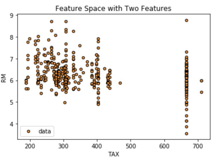
Just to make a point here, I simply filtered the dataset to two variables (TAX and RM). The plot below shows the feature space of those two variables, which was then segmented by the regression tree model. In reality, there were 13 variables, which make it very difficult to graphically show although I could have printed all bivariate combinations of the regressors in the model.
# Feature space with two regressors
plt.figure()
plt.scatter(X_train["TAX"], X_train["RM"], s=20, edgecolor="black", c="darkorange", label="data")
#plt.plot(X_test, predicted, color="cornflowerblue", label="max_depth=2", linewidth=2)

plt.xlabel("TAX")
plt.ylabel("RM")
plt.title("Feature Space with Two Features")
plt.legend()
plt.show()
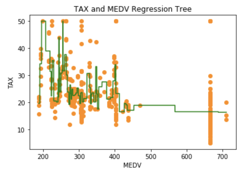
We can also illustrate how fitting a regression tree works by plotting actual observations and predicted values on the same plot. For simplicity, I selected a single variable (TAX) to demonstrate:
#Illustrate Regression Tree with a single regressor: TAX

#Filter all features but TAX and transfrom the dataframe to an array with [[]]
X_train2 = X_train['TAX']
X_tr2 = X_train2.values
X_tra2=X_tr2.reshape(404,-1)

#Fit regression tree
model100 = DecisionTreeRegressor(random_state=0)
model100.fit(X_tra2, y_ar)


#arange for creating a range of values  from min value of X_tra2 to max value of X_tra2
#These are the lowest and highest TAX values in the dataset
#use increments of 0.01

X_grid = np.arange(min(X_tra2), max(X_tra2), 0.01)

# reshape X_grid array into a single column
X_grid = X_grid.reshape((len(X_grid), 1))

# Create scatter plot - original observations
plt.scatter(X_tra2, y_ar, c="darkorange")

# plot predictions
plt.plot(X_grid, model100.predict(X_grid), color = 'green')

# Label plot
plt.title('TAX and MEDV Regression Tree')
plt.xlabel('MEDV')
plt.ylabel('TAX')

plt.show()
Tree Pruning:
The regression tree called model1 is probably not a great model because it was not pruned hence it is severely overfitted. As discussed earlier, it is a good idea to prune using cost complexity pruning. Unfortunately, sklearn does not have a tuning parameter (often referred to as alpha in other programming languages), but we can take care of tree pruning by tuning the max_depth parameter. There are several ways of accomplishing such a task….
First, some data wrangling is necessary. First, I wanted to restrict this demonstration to two variables for easier understanding, so I filtered the Boston Housing data to two regressors (TAX and RM). Second, the data frame needed to be converted into an array and then further processed so that each observation is a row and the column of the array represents a variable.
#filter for two variables from dataframe
X_train = X_train[['TAX','RM']]
X_test = X_test[['TAX', 'RM']]

#transfer arrays and reshape arrays of the features into a column
#Note that X_train has 404 observations and X_test has 202 observations
#Y_train has 404 observations and Y_test has 202 observations.

X_tr = X_train.values #transform data frame to array
X_te = X_test.values #transform data frame to array

X_tra=X_tr.reshape((404,-1)) #reshape array so that [[]] are used
X_tes=X_te.reshape((102,-1)) #reshape array so that [[]] are used

y_ar = Y_train.values #transform data frame to array
y_te = Y_test.values #transform data frame to array

y_tra=y_ar.reshape((404,-1)) #reshape array so that [[]] are used
y_tes=y_te.reshape((102,-1)) #reshape array so that [[]] are used
Cross Validation by Handwritten Code:
In the first example, I wrote a for loop that takes integers 1-20 and iterates by plugging them into the max_depth parameter. For each integer, a regression tree is fitted using the two features and the cross validation score is computed. The cross_valscore is available from sklearn. In this example, I specified r-squared as an evaluation criterion but there are several other options. Each is set up so that higher numbers mean a better model. Even errors are reported in a 1-error format so that a higher parameter can be considered better. The list can be found at Sci-Kit Learn.
I also decided to calculate the test error for each of the models. Both cross validation score and the test MSE lead to the same choice, e.g. the model is best with a maximum depth of 5 nodes. Note that the cross validation score output does not show the root and there are only 19 scores. The cross validation score is the highest at .61 and the test mean squared error is the lowest at 17.049901960784307 when the tree depth is five.
depth2=[]
for i in range(1,20):
    regressor2 = DecisionTreeRegressor(random_state=0, criterion="mae", max_depth=i)
    model2 = regressor2.fit(X_tra, y_ar)
    # Perform 5-fold cross validation
    model2_scores = cross_val_score(model2, X_tra, y_ar, cv = 5, scoring='r2')
    print("mean cross validation score: {}".format(np.mean(model2_scores)))
##########
    #Predict the response for test dataset
    y_pred2 = model2.predict(X_tes)
    depth2.append(mean_squared_error(y_te, y_pred2))
print(depth2)

mean cross validation score: 0.40473735132974
mean cross validation score: 0.554404151039055
mean cross validation score: 0.5725850756113022
mean cross validation score: 0.614474763103361
mean cross validation score: 0.6060067903631277
mean cross validation score: 0.5806216540832267
mean cross validation score: 0.5607525858971419
mean cross validation score: 0.48963924349410204
mean cross validation score: 0.4266329120998754
mean cross validation score: 0.43980330467950485
mean cross validation score: 0.42822877227418676
mean cross validation score: 0.3682594888866144
mean cross validation score: 0.367440322208621
mean cross validation score: 0.3342251894380832
mean cross validation score: 0.32527301665847913
mean cross validation score: 0.3165077458657656
mean cross validation score: 0.3252864476799817
mean cross validation score: 0.3335792135548522
mean cross validation score: 0.3322138314812365
[40.22872549019608, 23.84007352941176, 19.893823529411762, 20.853529411764704, 17.049901960784307, 18.08051470588235, 19.885857843137252, 19.723088235294117, 19.886691176470585, 22.79803921568628, 24.412965686274514, 47.8179656862745, 67.10276960784314, 67.33522058823532, 66.81083333333333, 67.52014705882353, 67.88017156862745, 67.14367647058825, 66.76995098039217]
Cross Validation with Grid Search:
It is possible to find max_depth by running GridSearchCV, which replaces the for loop in the prior example. In this case, the selected max_depth is four.
#Pruning with GridSearchCV
from sklearn.model_selection import GridSearchCV

parameters = {'max_depth':range(3,20)}
regressor3 = GridSearchCV(DecisionTreeRegressor(), parameters, n_jobs=4)
regressor3.fit(X=X_tra, y=y_ar)
tree_model = regressor3.best_estimator_
print (regressor3.best_score_, regressor3.best_params_)

0.5796528298078012 {'max_depth': 4}
Visualize the Regression Tree:
First, let us remember that at some point earlier, we filtered all regressors but TAX and RM, therefore the following model will be based on those two features. First, there will be no restrictions on the number of branches just to see what a tree would actually look like. Several new modules are necessary for the visualization, therefore it is important to load StringIO from sklearn, IPython.display and its Image component as well as pydotplus. The regression tree is rather wide and hard to see.
from sklearn.tree import export_graphviz
from sklearn.externals.six import StringIO
from IPython.display import Image
import pydotplus

dot_data = StringIO()
export_graphviz(model, out_file=dot_data,
                filled=True, rounded=True,
                special_characters=True)
graph = pydotplus.graph_from_dot_data(dot_data.getvalue())
graph.write_png('TAX.png')
Image(graph.create_png())

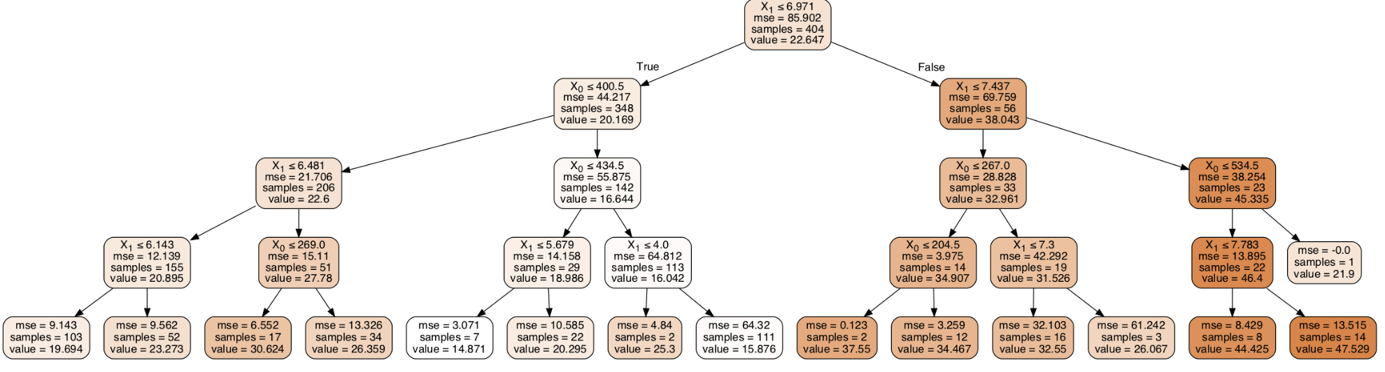
Let’s see what a pruned regression tree looks like now that we set the max_depth to four.
#An example of a regression tree with a maximum depth of only 4

# create a regressor object
regressor = DecisionTreeRegressor(random_state = 0, max_depth=4)
# fit the regressor with X_tra and y_ar data
model5=regressor.fit(X_tra, y_ar)

dot_data = StringIO()
export_graphviz(model5, out_file=dot_data,
                filled=True, rounded=True,
                special_characters=True)
graph = pydotplus.graph_from_dot_data(dot_data.getvalue())
graph.write_png('TAX.png')
Image(graph.create_png())
Understanding Regression Trees:
It is possible to inquire about the regression tree structure with Python by examining an attribute of the tree estimator called tree_ . The binary tree tree_ contains parallel arrays. The following can be viewed according to Sci-Kit Learn:
the binary tree structure;
the depth of each node and whether or not it’s a leaf;
the nodes that were reached by a sample using the
decision_pathmethod;the leaf that was reached by a sample using the apply method;
the rules that were used to predict a sample;
the decision path shared by a group of samples.
The i-th element of each array holds information about the node `i`. Node 0 is the tree's root. NOTE: Some of the arrays only apply to either leaves or split nodes, resp. In this . case the values of nodes of the other type are arbitrary!
#Understand the structure of a tree
regressor = DecisionTreeRegressor(max_depth=2, random_state=0)
regressor.fit(X_tra, y_ar)

# Use arrays to examine tree structure
n_nodes = regressor.tree_.node_count
children_left = regressor.tree_.children_left
children_right = regressor.tree_.children_right
feature = regressor.tree_.feature
threshold = regressor.tree_.threshold
print(n_nodes)
print ('number of nodes:', n_nodes)
print('children left', children_left)
print('children right',children_right)
print('feature', feature)
print('threshold', threshold)

number of nodes: 29
children left [ 1  2  3  4 -1 -1  7 -1 -1 10 11 -1 -1 14 -1 -1 17 18 19 -1 -1 22 -1 -1
 25 26 -1 -1 -1]
children right [16  9  6  5 -1 -1  8 -1 -1 13 12 -1 -1 15 -1 -1 24 21 20 -1 -1 23 -1 -1
 28 27 -1 -1 -1]
feature [ 1  0  1  1 -2 -2  0 -2 -2  0  1 -2 -2  1 -2 -2  1  0  0 -2 -2  1 -2 -2
  0  1 -2 -2 -2]
threshold [  6.97149992 400.5          6.48149991   6.14300013  -2.
  -2.         269.          -2.          -2.         434.5
   5.67949986  -2.          -2.           4.00049996  -2.
  -2.           7.43700004 267.         204.5         -2.
  -2.           7.30000019  -2.          -2.         534.5
   7.78349996  -2.          -2.          -2.        ]
A lot of the information coming from these arrays can be seen on the tree plot. For example, there are 29 nodes. One can count them on the tree plot as well. The i-th element of each # array holds information about the node `i`. I find this incredibly useful for interpretation especially of the nodes on a tree plot are very small and hard to see.
# compute depth of each node
# identify if it is a leaf.
node_depth = np.zeros(shape=n_nodes, dtype=np.int64)
is_leaves = np.zeros(shape=n_nodes, dtype=bool)
stack = [(0, -1)]  # seed is the root node id and its parent depth
while len(stack) > 0:
    node_id, parent_depth = stack.pop()
    node_depth[node_id] = parent_depth + 1

    # If we have a test node
    if (children_left[node_id] != children_right[node_id]):
        stack.append((children_left[node_id], parent_depth + 1))
        stack.append((children_right[node_id], parent_depth + 1))
    else:
        is_leaves[node_id] = True
print("The binary tree structure has %s nodes and has "
      "the following tree structure:"
      % n_nodes)
for i in range(n_nodes):
    if is_leaves[i]:
        print("%snode=%s leaf node." % (node_depth[i] * "\t", i))
    else:
        print("%snode=%s test node: go to node %s if X[:, %s] <= %s else to "
              "node %s."
              % (node_depth[i] * "\t",
                 i,
                 children_left[i],
                 feature[i],
                 threshold[i],
                 children_right[i],
                 ))
print()
The binary tree structure has 29 nodes and has the following tree structure:
node=0 test node: go to node 1 if X[:, 1] <= 6.971499919891357 else to node 16.
    node=1 test node: go to node 2 if X[:, 0] <= 400.5 else to node 9.
        node=2 test node: go to node 3 if X[:, 1] <= 6.481499910354614 else to node 6.
            node=3 test node: go to node 4 if X[:, 1] <= 6.14300012588501 else to node 5.
                node=4 leaf node.
                node=5 leaf node.
            node=6 test node: go to node 7 if X[:, 0] <= 269.0 else to node 8.
                node=7 leaf node.
                node=8 leaf node.
        node=9 test node: go to node 10 if X[:, 0] <= 434.5 else to node 13.
            node=10 test node: go to node 11 if X[:, 1] <= 5.679499864578247 else to node 12.
                node=11 leaf node.
                node=12 leaf node.
            node=13 test node: go to node 14 if X[:, 1] <= 4.000499963760376 else to node 15.
                node=14 leaf node.
                node=15 leaf node.
    node=16 test node: go to node 17 if X[:, 1] <= 7.437000036239624 else to node 24.
        node=17 test node: go to node 18 if X[:, 0] <= 267.0 else to node 21.
            node=18 test node: go to node 19 if X[:, 0] <= 204.5 else to node 20.
                node=19 leaf node.
                node=20 leaf node.
            node=21 test node: go to node 22 if X[:, 1] <= 7.300000190734863 else to node 23.
                node=22 leaf node.
                node=23 leaf node.
        node=24 test node: go to node 25 if X[:, 0] <= 534.5 else to node 28.
            node=25 test node: go to node 26 if X[:, 1] <= 7.7834999561309814 else to node 27.
                node=26 leaf node.
                node=27 leaf node.
            node=28 leaf node.

