

Ensemble Methods: Boosting

““Thank you for leaving us alone but giving us enough attention to boost our egos.””
Objectives:
Demonstrate how to build models with Gradient Boosting, Extreme Gradient Boosting and Adaptive Boosting methods;
Show how to tune parameters of boosting models by cross validation; and
Learn how to tune parameters of boosting models using grid search and cross validation.
Boosting:
Boosting is also an ensemble method based on regression trees. During boosting a sequence of trees is grown and successive trees are cultivated on the residuals of preceding trees. Note that during boosting, residuals are used, not the dependent variable for sequential tree fitting. When boosting, bootstrapping is not used but each tree is fit on the original data set. When the next sequence of trees is built, the residuals are updated. Boosting uses three main tuning parameters: the number of trees, a shrinkage parameter and the number of splits per tree. Cross-validation should be used to decide on the number of trees. The shrinkage parameter is usually a small number (0.01 or 0.001), and must be evaluated in the context of the number of trees used because a very small shrinkage parameter typically requires a large number of trees. The number of splits in each tree is used to control the complexity of the ensemble model. It is often sufficient to create a tree stump by setting this parameter to one.
Types of Boosting:
Several versions of boosting are available for ensemble learning: (a) Adaptive Boosting, (b) Gradient Boosting, (c) Extreme Gradient Boosting, and (d) Light GBM.
Adaptive Boosting Regressor:
A meta-estimator, AdaBoost begins by fitting a regressor on the original dataset and continues to fit additional copies of the regressor on the same dataset. The weights of instances are adjusted according to the error of current prediction. The predictions are combined by using a weighted majority vote. Incorrect predictions by the boosted model have their weights increased at each step, while correct predictions are assigned lower weights. Difficult to predict observations have a larger influence as a result.
Gradient Boosting Regressor:
Gradient boosting is a generalization of boosting to a loss function (the default is least squares). The method uses several weak learners (e.g. individual regression trees) that are combined to form a strong learner (e.g. the ensemble of regression trees). The number of weak learners for ensemble learning can be specified by the parameter n_estimators. Also, the size of each weak learner can be pre-determined two different ways: by specifying tree depth (max_depth) or setting the number of leaf nodes (max_leaf_nodes). The learning rate is the shrinkage parameter, which controls overfitting and ranges between 0.0 and 1.0. Regression trees are first grown as the base learner, and subsequent tree ensembles are grown using the errors of the prior trees.
Extreme Boosting Regressor:
XG Boost works similarly to the gradient boosting regressor, but it is designed to achieve better training speed because of memory efficiency. Before first use, it must be installed from a terminal window. I use Anaconda, which requires conda install -c anaconda py-xgboost.
A really important point is that XG Boost uses an optimized data structure called Dmatrix, which must be created before XG Boost can be trained.
Applied Boosting:
In order to demonstrate how to create boosted models, we need to load specific libraries. We also need to ingest the Boston Housing data set.
import numpy as np
import matplotlib.pyplot as plt
import pandas as pd

import sklearn
from sklearn.ensemble import GradientBoostingRegressor
from sklearn.ensemble import AdaBoostRegressor
from sklearn.tree import DecisionTreeRegressor
from sklearn.model_selection import ParameterGrid
from sklearn import ensemble
from sklearn.metrics import mean_squared_error
from sklearn.model_selection import GridSearchCV
from sklearn.utils import shuffle

from sklearn.datasets import load_boston
boston= load_boston()
boston_features_df = pd.DataFrame(data=boston.data,columns=boston.feature_names)
boston_target_df = pd.DataFrame(data=boston.target,columns=['MEDV'])
X_train, X_test, y_train, y_test = sklearn.model_selection.train_test_split(boston_features_df, boston_target_df, test_size = 0.20, random_state = 5
The next task is to transform the data frames of the partitioned Boston Housing data into arrays. Take notice of revel(), which was necessary to create a one dimensional array. When the data y_train and y_test data frames were originally transformed into arrays, they were two dimensional, although they contained only one column, while the other column of the array was empty. This issue was solved by revel()
#create arrays
#use ravel() for y_test and y_train to align with one dimensional array expectation
X_tra=X_train.values
X_tes=X_test.values
y_tra=y_train.values.ravel()
y_tes=y_test.values.ravel()
Applied Gradient Boosting:
The first method we look at is gradient boosting. I set up a grid for tuning several parameters. In this example, tuning was done iteratively. For each parameter, a minimum and maximum value was selected that were reasonably far from each other. The mid-point between these two values was also indicated. The three points were then used to fit boosted models. In this example, there were three parameters tuned: n_estimators and max_depth had three levels each, while min_samples_split had two levels. As a result, (3*3*2) 18 models were fitted with all combinations of indicated parameters and parameter levels. For each model, the test MSE was computed to aid the selection of the best model.
The iterative nature of parameter selection is due to the selection of parameter values based on three anchors. For example, n_estimators has three levels: 500, 750 and 1000. After finding the model with the lowest test MSE among the 18 candidate models, we can check which of the three levels were used by the champion model. We can then change the levels of n_estimator by selecting the winning level and its closest level as the new minimum and maximum, enter the mid-point between them and try to refit the model. We can iterate, until we don’t see an improvement in the test MSE. Note that later we will look at grid search, (GridSearchCV) which may be a better approach.
#############################
#Gradient Boosting with simple grid
#Only three parameters tuned, all others kept as default
grid = ParameterGrid({'n_estimators':[500, 750, 1000], 'max_depth': [1,  2, 3],'min_samples_split':  [0.1, 0.15], })

for parameters in grid:
    regressor=ensemble.GradientBoostingRegressor(**parameters, random_state=123, learning_rate= 0.1)
    model=regressor.fit(X_tra, y_tra)
    y_pred = model.predict(X_tes)

    #compute MSE
    mse = mean_squared_error(y_tes, y_pred)
    print("MSE: %.2f" % mse)

    #Show tuned parameters for each iteration (3*3*2 models)
    tuned_parameters=model.get_params
    print(tuned_parameters)
The winning model had a test MSE of 7.05 and selected the following tuned levels for the three parameters:
n_estimators = 750
max_depth = 2
min_samples_split = 0.1
MSE: 7.05
<bound method BaseEstimator.get_params of GradientBoostingRegressor(alpha=0.9, criterion='friedman_mse', init=None,
                          learning_rate=0.1, loss='ls', max_depth=2,
                          max_features=None, max_leaf_nodes=None,
                          min_impurity_decrease=0.0, min_impurity_split=None,
                          min_samples_leaf=1, min_samples_split=0.1,
                          min_weight_fraction_leaf=0.0, n_estimators=750,
                          n_iter_no_change=None, presort='auto',
                          random_state=123, subsample=1.0, tol=0.0001,
                          validation_fraction=0.1, verbose=0, warm_start=False)>
We can plot the accuracy of our model using the training and test data. We can observe that deviation drops quickly as we increase n_estimators(the number of trees used during boosting) but stays relatively stable as n_estimators increases.
# #############################################
# Plot accuracy of test and training
# compute test set deviance
test_score = np.zeros((parameters['n_estimators'],), dtype=np.float64)

for i, y_pred in enumerate(model.staged_predict(X_tes)):
    test_score[i] = model.loss_(y_tes, y_pred)

plt.figure(figsize=(22, 4))
plt.subplot(1, 2, 1)
plt.title('Accuracy Expressed as Devience')
plt.plot(np.arange(parameters['n_estimators']) + 1, model.train_score_, 'g-',
         label='Training Set Deviance')
plt.plot(np.arange(parameters['n_estimators']) + 1, test_score, 'r-',
         label='Test Set Deviance')
plt.legend(loc='upper right')
plt.xlabel('n_estimators')
plt.ylabel('Deviance')

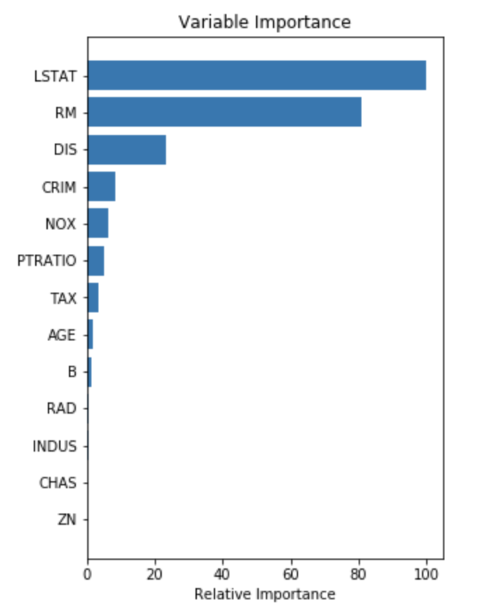
Another very useful plot from boosting is the feature importance plot. The measures are based on the number of times a variable is selected for splitting, weighted by the squared improvement to the model as a result of each split, and averaged over all trees. [Elith et al. 2008, A working guide to boosted regression trees]
# #####################
# Plot feature importance
names=X_train.columns.values #get column header from training features

feature_importance = model.feature_importances_
# make importances relative to max importance
feature_importance = 100.0 * (feature_importance / feature_importance.max())
sorted_idx = np.argsort(feature_importance)
pos = np.arange(sorted_idx.shape[0]) + .5
plt.subplot(2, 2, 2)
plt.barh(pos, feature_importance[sorted_idx], align='center')
plt.yticks(pos, names[sorted_idx])

plt.xlabel('Relative Importance')
plt.title('Variable Importance')
plt.show()
Parameter Tuning with GridSearch CV:
Now let’s turn to a more thorough approach to parameter tuning: tune with GridSearch CV. The approach requires us to set up an estimator and a parameter grid.
#################################
#Parameter tuning with GridSearchCV (still Gradient Boosting)
estimator = ensemble.GradientBoostingRegressor( random_state=0, learning_rate= 0.1)

set up parameters to be tuned
parameters = {
    'max_depth': range (1, 3, 1),
    'n_estimators': range(740, 760, 5),
    'learning_rate': [0.01, 0.2, 0.01],
    'min_samples_split':  [0.01, 0.2, 0.01],
}

#Gradient boosting with GridSearchCV
grid_search = GridSearchCV(
    estimator=estimator,
    param_grid=parameters,
    scoring = 'neg_mean_squared_error',
    n_jobs = 10,
    cv = 5,
    verbose=True)

grid_search.fit(X_train, y_train)
We need to get the information stored in various objects (depending on what we are looking for. Here, I wanted to show, the tuned parameters and the model score for decision making.
#print key model parameters
a=grid_search.best_estimator_  #shows the model's parameters
b=grid_search.best_params_     #shows tuned parameters
c=grid_search.best_score_      #shows best model's score (lower is better)
print(a)
print(b)
print(c)
The resulting code shows that the three parameters were tuned a bit differently vs.when we tuned them by hand. Note that I also added a fourth parameter to tune, learning_rate. The resulting model score was -11.991046150523072.
n_estimators = 745
max_depth = 2
min_samples_split = 0.01
learning_rate: 0.2
GradientBoostingRegressor(alpha=0.9, criterion='friedman_mse', init=None,
                          learning_rate=0.2, loss='ls', max_depth=2,
                          max_features=None, max_leaf_nodes=None,
                          min_impurity_decrease=0.0, min_impurity_split=None,
                          min_samples_leaf=1, min_samples_split=0.01,
                          min_weight_fraction_leaf=0.0, n_estimators=745,
                          n_iter_no_change=None, presort='auto', random_state=0,
                          subsample=1.0, tol=0.0001, validation_fraction=0.1,
                          verbose=0, warm_start=False)
{'learning_rate': 0.2, 'max_depth': 2, 'min_samples_split': 0.01, 'n_estimators': 745}
-11.991046150523072
The model scores are helpful to compare the performance of a model to that of others. Best score is the mean cross-validated score. I still wanted to calculate the test MSE of the champion model: which turned out to be 7.06. (Note that the available levels for each parameter are still restricted by the minimum and maximum and the the allowed step size in grid search. These were somewhat different than the parameter levels in the hand tuned model. )
#############################
#Compute test MSE: Gradient Boosting
#Change parameter's default to best_params_ values and re-run model.

regressor=ensemble.GradientBoostingRegressor(alpha=0.9, criterion='friedman_mse', init=None,
                          learning_rate=0.2, loss='ls', max_depth=2,
                          max_features=None, max_leaf_nodes=None,
                          min_impurity_decrease=0., min_impurity_split=None,
                          min_samples_leaf=1, min_samples_split=0.01,
                          min_weight_fraction_leaf=0.0, n_estimators=745,
                          n_iter_no_change=None, presort='auto', random_state=0,
                          subsample=1.0, tol=0.0001, validation_fraction=0.1,
                          verbose=0, warm_start=False)
model=regressor.fit(X_tra, y_tra)
y_pred = model.predict(X_tes)

#compute MSE
mse = mean_squared_error(y_test, y_pred)
print("MSE: %.2f" % mse)

#Compute RMSE
rmse = np.sqrt(mean_squared_error(y_test, y_pred))
print("RMSE: %f" % (rmse))
Applied Adaptive Boosting:
Adaptive boosting can be executed the same way as gradient boosting. I wanted to see how the AdaBoostRegressor performs vs. the GradientBoostRegressor, therefore I placed the same constraints on parameters as in the prior example for gradient boosting. Generally, all test MSE scores were higher than the champion gradient boosted model's MSE.
#############################
#Adaptive Boosting with simple grid
grid = ParameterGrid({'n_estimators':[740, 745, 750],
                          'learning_rate': [0.1,  0.2],
                          'loss' : ['linear']
                         })
for params in grid:
    ada_regressor=ensemble.AdaBoostRegressor(**params, random_state=0)
    ada_model=ada_regressor.fit(X_tra, y_tra)
    y_pred = ada_model.predict(X_tes)

    #compute MSE
    mse = mean_squared_error(y_tes, y_pred)
    print("MSE: %.2f" % mse)

    parameters=ada_model.get_params
    print(parameters)
Applied Extreme Gradient Boosting:
XG Boost uses parallel processing and is designed to handle missing values and offers regularization to achieve superior predictions of categorical and continuous targets alike. XG Boost is not part of the Sci-Kit learn and must be installed separately first. Once installed, it does work well with components of sklearn. As discussed earlier, XB Boost utilizes D-matrix, which must be specified before model fitting.
######################
#XG Boost
import xgboost as xgb
data_dmatrix = xgb.DMatrix(data=X_tra,label=y_tra) #matrix is important component for XG Boost
XG Boost allows the tuning of several parameters. Some of them were available in gradient boosting models as well.
learning_rate: step size shrinkage ranging between 0 and 1.
max_depth: specifies the depth of each tree.
subsample: is a percentage of samples used in any given tree
colsample_bytree: is the percentage of features used in any given tree.
n_estimators: determines the number of trees built.
objective: determines the loss function and will be set to linear, since the current model is a regression model.
Regularization is also a feature of XG Boost. Several options are available and they are tunable.
gamma: determines if a node is allowed to split
alpha: L1 regularization on leaf weights.
lambda: a smoother L2 regularization on leaf weights
The below demonstrates how XG Boots models are specified. Note the parameters to be tuned later. Predictions are also made and the test MSE/RMSE are computed.
xg_regressor = xgb.XGBRegressor(objective ='reg:linear', colsample_bytree = 0.4, learning_rate = 0.3, max_depth = 5,
                                alpha = 4, n_estimators = 8)
xg_regressor.fit(X_train,y_train)
preds = xg_regressor.predict(X_test)
#compute MSE
mse = mean_squared_error(y_test, preds)
print("MSE: %.2f" % mse)

#compute RMSE
rmse = np.sqrt(mean_squared_error(y_test, preds))
print("RMSE: %f" % (rmse))
XG Boost with Cross-validation:
In order to tune the parameters, cross-validation can be used. Cross-validation is done using cv(), where the nfolds parameter specifies the number of cross-validation sets. As a general good practice, the seed should be set to reproduce the results. A dictionary called parameters was also created which contains the parameters to be tuned. The resulting cv_results contains the RMSE score of each boosting round. The last entry contains the best model, since it has the lowest RMSE, in this case 3.814772. .
#Cross validation
parameters = {"objective":"reg:linear",'colsample_bytree': 0.2,'learning_rate': 0.1,
                'max_depth': 5, 'alpha': 4}

cv_results = xgb.cv(dtrain=data_dmatrix, params=parameters, nfold=5,
                    num_boost_round=200,early_stopping_rounds=10,metrics="rmse", as_pandas=True, seed=123)
cv_results.head(5)
#len(cv_results)
#Show RMSE
print((cv_results["test-rmse-mean"]).tail(5))

195    3.816269
196    3.815869
197    3.815914
198    3.814771
199    3.81477
GridSearchCV to Tune XG Boost Parameters:
The result can be further improved by using GridSearchCV to tune model parameters. In fact, the best model contains the following parameters specified:
learning_rate: 0.2,
max_depth: 2,
n_estimators: 190
#######################################
#Parameter tuning with GridSearch
regressor_xgb = xgb.XGBRegressor(objective= 'reg:linear', nthread=4, seed=2)
###
parameters = {
    'max_depth': range (2, 3, 1),
    'n_estimators': range(190, 200, 5),
    'learning_rate': [0.2, 0.25, 0.01]
}
grid_search = GridSearchCV(
    estimator=regressor_xgb,
    param_grid=parameters,
    scoring = 'neg_mean_squared_error',
    n_jobs = 10,
    cv = 3,
    verbose=True)
grid_search.fit(X_tra, y_tra)
a=grid_search.best_estimator_
b=grid_search.best_params_
c=grid_search.best_score_
print(a)
print(b)
print(c)

XGBRegressor(base_score=0.5, booster='gbtree', colsample_bylevel=1,
             colsample_bynode=1, colsample_bytree=1, gamma=0,
             importance_type='gain', learning_rate=0.2, max_delta_step=0,
             max_depth=2, min_child_weight=1, missing=None, n_estimators=190,
             n_jobs=1, nthread=4, objective='reg:linear', random_state=0,
             reg_alpha=0, reg_lambda=1, scale_pos_weight=1, seed=2, silent=None,
             subsample=1, verbosity=1)
{'learning_rate': 0.2, 'max_depth': 2, 'n_estimators': 190}
-12.290093813109372
If we take the champion model’s parameter levels we can calculate the test MSE of the resulting model. In fact, the test MSE turned out to be 6.96 and the test RMSE was 2.64. Remember that cross validation helped us to an RMSE score of 3.81, therefore grid search and cross validation aided model performance significantly. Depending on ambition and time, the model can be further optimized.
#### Calculate the actual test MSE for comparison with other models
xg_regression = xgb.XGBRegressor(base_score=0.5, booster='gbtree', colsample_bylevel=1,
             colsample_bynode=1, colsample_bytree=1, gamma=0,
             importance_type='gain', learning_rate=0.2, max_delta_step=0,
             max_depth=2, min_child_weight=1, missing=None, n_estimators=190,
             n_jobs=1, nthread=4, objective='reg:linear', random_state=0,
             reg_alpha=0, reg_lambda=1, scale_pos_weight=1, seed=2, silent=None,
             subsample=1, verbosity=1)
xg_regression.fit(X_train,y_train)
preds = xg_regression.predict(X_test)

#compute MSE
mse = mean_squared_error(y_test, preds)
print("MSE: %.2f" % mse)

#compute RMSE
rmse = np.sqrt(mean_squared_error(y_test, preds))
print("RMSE: %f" % (rmse))
Visualize XG Boost Models:
Feature importance plots are available in XG Boost as well. They represent the same idea as with other boosting models.
xgb.plot_importance(xg_reg)
plt.figure(num=None, figsize=(8, 6), dpi=80, facecolor='w', edgecolor='k')
plt.show()

Finally, here’s the boosted model structure graphically explained.
import matplotlib.pyplot as plt

xgb.plot_tree(xg_reg,num_trees=0)
plt.rcParams['figure.figsize'] = [150, 10]
plt.show()


