

Regularization and Shrinkage: Ridge, Lasso and Elastic Net Regression

““Water shrinks wool, urgency shrinks time.
Shrinkage may be an advantage or the reverse, according to expectation.””
Objectives:
Introduce shrinkage methods in regression analysis;
Explain how ridge, lasso and elastic net regression work;
Discuss the similarities and differences in shrinkage (L1, L2 and L1+L2 penalties);
Demonstrate the impact of penalty terms on model accuracy;
Use Sci-Kit (sklearn) machine learning library to fit penalized regression models with Python
Show how to use cross validation to find the shrinkage parameter (λ) in ridge and lasso and the L1/L2 ratio in elastic net.
Background:

OLS Regression: The equation is the basic representation of the relationship between a response (Y) and several predictor variables (here shown as X1,X2,...,Xp.)
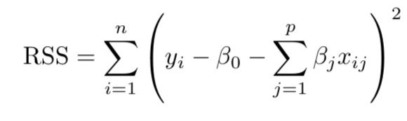
Several other approaches are available that extend the linear approach: we simply we need to change the fitting method of OLS. In fact, some of these models (ridge, lasso and elastic net regression) may provide better accuracy on test data and may help us interpret model outputs better. In this post, the discussion is centered around shrinkage methods, which constrain the parameter estimates by reducing the variance albeit at the minor cost of increased bias. In many cases, model accuracy on test data improves a great deal. In all cases, penalized regression models are extensions of the OLS model where the goal was to minimize RSS or residual sum of squares:
What is shrinkage?
Shrinkage means that the coefficients are reduced towards zero compared to the OLS parameter estimates. This is called regularization. Since the lowest possible estimate for a coefficient is zero, some – but not all - of the regularization models may be used for parameter selection (more about this later.)
Ridge Regression:
When estimating coefficients in ridge regression, we minimize the following equation. Note λ (a tuning parameter) which is a value greater than or equal to zero. The second term containing lambda acts as the shrinkage penalty. The goal is - similar to least squares estimates - still to minimize RSS.
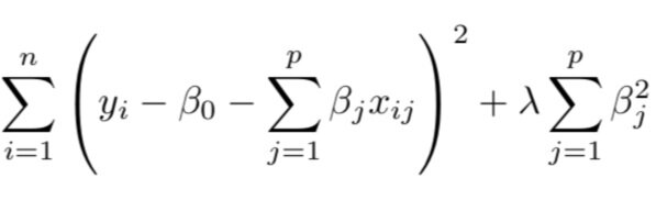
When lambda is 0, the penalty has no impact, and the model fitted is an OLS regression. However, when lambda is approaching infinity, the shrinkage penalty becomes very large and coefficient estimates will have a zero value. Therefore, estimating lambda is very important, and can be effectively done using cross-validation. Also, the shrinkage is not applied to the intercept.
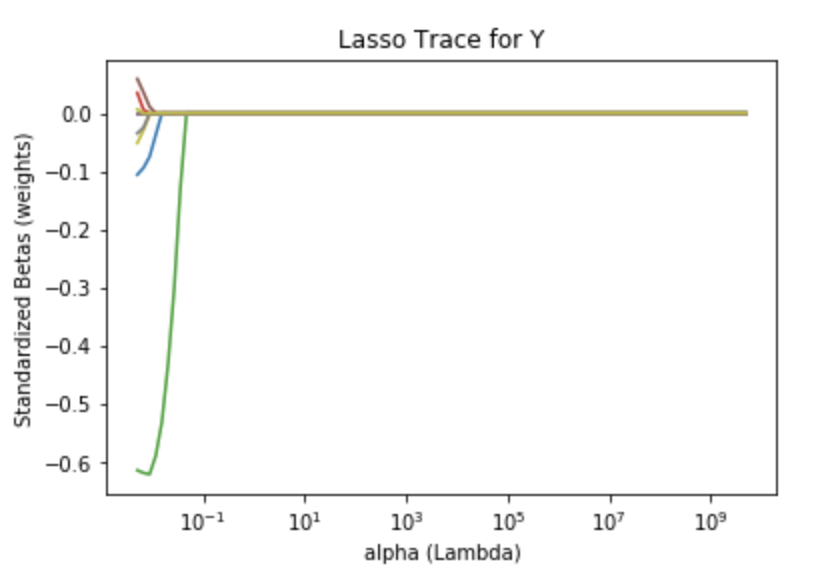
The plot below shows ridge regression coefficients against the shrinkage penalty. Each curve represents one of the 29 variables. The left part of the plot shows OLS estimates, and lambda starts shrinking the parameter estimates at a differential rate as one moves towards the right. At the right-hand side of the plot all estimates become zero and there are no parameters in the model. In fact, coefficient estimates become zero before λ reaches the value 10.

Coefficients depend not only on the shrinkage parameter but also on the scaling of other parameters. Shrinkage may change the parameter estimate by a very large factor, therefore the standardization of regressors is important. Sci-kit can do this automatically.
In reality, ridge regression will always include all predictors, because the penalty (λ) will never reach exactly zero. Lambda would have to equal infinity for the coefficient to be shrunk to zero, which typically does not happen. As a result, a large number of variables may make it difficult to interpret when ridge regression is used.
Lasso Regression (Least Absolute Shrinkage and Selection Operator):
The lasso regression may serve as a good alternative to ridge regression because it allows for coefficients to be set to zero. When fitting a lasso model, the goal is to minimize the quantity expressed by the equation below. It is very similar to the ridge equation except that it uses a different penalty term, an L1 instead of an L2 penalty. If we examine the difference, we discover that ridge regression has a βj2 term, while the lasso has a |βj | term in the penalty. With the alternative penalty term, the lasso can shrink the coefficients to be exactly zero if lambda is large. A result, the lasso may be used for variable selection and the resulting. Models can be easily interpreted even when a large number of variables were originally used when fitting the model.

The plot below shows lasso regression coefficients against the shrinkage penalty. Again, each curve represents one of the 29 variables. As a result of the alternate shrinkage penalty, the plot shows a different picture of how parameter estimates become zero as we increase λ.
Elastic Net:
Elastic net regression combines the penalty terms of ridge and lasso regression. When fitting models with elastic net, we minimize the function:

In this model, we have an additional parameter referred to as mixing parameter or α which is designed to mix the penalties from the two different shrinkage parameters, ridge (α = 0) and lasso (α = 1).
In this case, we need to tune two parameters, λ and α when computing the penalty term, and the task can be accomplished by cross validation .
The plot below shows elastic net coefficients against the shrinkage penalty. Again, each curve represents one of the 29 variables. Here both λ and α are tuned .

How to select the tuning parameter:
The best way to select a lambda value for tuning is to create a grid of lambda values and then perform cross validation on each. Select the value for which the cross validation error is minimal.
So let’s see what penalized regression looks like with sklearn. First, load all necessary libraries, and load the dataset: boston.
import pandas as pd
import statsmodels.api as sm
import numpy as np
import sklearn

%matplotlib inline
import matplotlib.pyplot as plt
from sklearn.linear_model import Ridge, RidgeCV, Lasso, LassoCV, ElasticNet, ElasticNetCV

from sklearn.metrics import mean_squared_error
from sklearn.linear_model import Ridge
from sklearn.preprocessing import StandardScaler
from sklearn.preprocessing import PolynomialFeatures
from sklearn.preprocessing import scale
#load and partition data
from sklearn.datasets import load_boston
boston= load_boston()

boston_features_df = pd.DataFrame(data=boston.data,columns=boston.feature_names)
boston_target_df = pd.DataFrame(data=boston.target,columns=['MEDV'])
The next step is to transform the data. The box-cox method was used. Since some of the variables contained 0s, I added 1 to every value in the dataset.
#Transform data
#add one to each value to get rid of 0 values in both target and features

numeric_cols = [col for col in boston_features_df if boston_features_df[col].dtype.kind != 'O']
numeric_cols
numeric_cols2 = [col for col in boston_target_df if boston_target_df[col].dtype.kind != 'O']
numeric_cols2

boston_features_df[numeric_cols] += 1
boston_target_df[numeric_cols2] += 1
boston_features_df.head()
boston_target_df.head()

#Use box-cox transformation
import pandas as pd
import numpy as np
from sklearn.preprocessing import StandardScaler
from sklearn.compose import ColumnTransformer
from sklearn.preprocessing import PowerTransformer

#Box-Cox Transform features
column_trans = ColumnTransformer(
    [('CRIM_bc', PowerTransformer(method='box-cox', standardize=True), ['CRIM']),
     ('ZN_bc', PowerTransformer(method='box-cox', standardize=True), ['ZN']),
     ('INDUS_bc', PowerTransformer(method='box-cox', standardize=True), ['INDUS']),
     ('CHAS_bc', PowerTransformer(method='box-cox', standardize=True), ['CHAS']),
     ('NOX_bc', PowerTransformer(method='box-cox', standardize=True), ['NOX']),
     ('RM_bc', PowerTransformer(method='box-cox', standardize=True), ['RM']),
     ('AGE_bc', PowerTransformer(method='box-cox', standardize=True), ['AGE']),
     ('DIS_bc', PowerTransformer(method='box-cox', standardize=True), ['DIS']),
     ('RAD_bc', PowerTransformer(method='box-cox', standardize=True), ['RAD']),
     ('TAX_bc', PowerTransformer(method='box-cox', standardize=True), ['TAX']),
     ('PTRATIO_bc', PowerTransformer(method='box-cox', standardize=True), ['PTRATIO']),
     ('B_bc', PowerTransformer(method='box-cox', standardize=True), ['B']),
     ('LSTAT_bc', PowerTransformer(method='box-cox', standardize=True), ['LSTAT']),
    ])

transformed_boxcox = column_trans.fit_transform(boston_features_df)
new_cols = ['CRIM_bc', 'ZN_bc', 'INDUS_bc', 'CHAS_bc', 'NOX_bc', 'RM_bc', 'AGE_bc', 'DIS_bc','RAD_bc','TAX_bc','PTRATIO_bc', 'B_bc', 'LSTAT_bc']

boston_features_bc = pd.DataFrame(transformed_boxcox, columns=new_cols)
pd.concat([ boston_features_bc], axis = 1)
boston_features_bc.head()

##### Box-Cox tranform target
column_trans = ColumnTransformer(
    [('MEDV_bc', PowerTransformer(method='box-cox', standardize=True), ['MEDV']),
    ])
transformed_boxcox = column_trans.fit_transform(boston_target_df)
new_cols2 = ['MEDV_bc']

boston_target_bc = pd.DataFrame(transformed_boxcox, columns=new_cols2)
pd.concat([ boston_target_bc], axis = 1)
boston_target_bc.head()
Now that both features and the target have been transformed, the dataset was partitioned into train and test sets.
#Partition the data based on box-cox transformed dataframes
X = boston_features_bc
Y = boston_target_bc
X_train, X_test, Y_train, Y_test = sklearn.model_selection.train_test_split(X, Y, test_size = 0.20, random_state = 5)
X_train.head(3)
| CRIM_bc | ZN_bc | INDUS_bc | CHAS_bc | NOX_bc | RM_bc | AGE_bc | DIS_bc | RAD_bc | TAX_bc | PTRATIO_bc | B_bc | LSTAT_bc | |
|---|---|---|---|---|---|---|---|---|---|---|---|---|---|
| 33 | 0.431336 | -0.599954 | -0.261894 | -0.272599 | 0.0227165 | -0.824820 | 0 | -0.008199 | 0.345251 | -0.025494 | 0.141112 | -0.161930 | -0.042164 |
| 283 | -1.032587 | 1.730203 | -1.905230 | 3.668398 | -1.639940 | 2.215613 | -1.515715 | 1.093848 | -2.314674 | -1.861545 | -1.792346 | 0.588025 | -1.849143 |
| 418 | 1.781079 | -0.599954 | 1.010936 | -0.272599 | 0.0227165 | -0.824820 | 0 | -0.008199 | 0.345251 | 1.369662 | 0.838670 | -2.797482 | 1.126252 |

The next step was to create polynomial terms and interaction terms. For simplicity, I only created second degree polynomials. Also, prior analysis revealed which interactions may provide additional benefit to the model, therefore only those deemed important were kept for further analysis. (See Interaction Effects and Polynomials in Multiple Regression on Datasklr.com) . There were a 104 columns retained.
# Create interaction terms (interaction of each regressor pair + polynomial)
#Interaction terms need to be created in both the test and train datasets
interaction = PolynomialFeatures(degree=2, include_bias=False, interaction_only=False)

#X traning
#Note the use of input_features=boston.feature_names which switches back to nomenclature without _bc
X_interact_train = pd.DataFrame(interaction.fit_transform(X_train), columns=interaction.get_feature_names(input_features=boston.feature_names))
print(X_interact_train.head(3))

#X test
#Note the use of input_features=boston.feature_names which switches back to nomenclature without _bc
X_interact_test = pd.DataFrame(interaction.fit_transform(X_test), columns=interaction.get_feature_names(input_features=boston.feature_names))

#Since X_inter is used in regression, the index of the that dataset and the outcome variable must be the same
#Reset the index of Y manually
#Y training
Y_interact_train=Y_train.reset_index()
Y_interact_train=Y_interact_train.drop(['index'], axis=1)

#Y test
Y_interact_test=Y_test.reset_index()
Y_interact_test=Y_interact_test.drop(['index'], axis=1)
print(Y_interact_test.head(3))
CRIM ZN INDUS CHAS NOX RM AGE \ 0 0.431336 -0.599954 -0.261894 -0.272599 0.027165 -0.824820 0.977600 1 -1.032587 1.730203 -1.905230 3.668398 -1.639940 2.215613 -1.515715 2 1.781079 -0.599954 1.010936 -0.272599 1.120349 -0.443073 1.192354 DIS RAD TAX TAX^2 TAX PTRATIO TAX B \ 0 0.300833 -0.529331 -0.450925 0.203334 -0.645141 0.204302 1 1.093848 -2.314674 -1.861545 3.465348 3.336532 -1.094634 2 -1.130511 1.446832 1.369662 1.875973 1.148694 -3.831605 TAX LSTAT PTRATIO^2 PTRATIO B PTRATIO LSTAT B^2 B LSTAT \ 0 -0.406499 2.046916 -0.648214 1.289749 0.205276 -0.408436 1 3.442261 3.212504 -1.053944 3.314303 0.345773 -1.087342 2 1.542584 0.703368 -2.346165 0.944554 7.825908 -3.150669 LSTAT^2 0 0.812662 1 3.419328 2 1.268443 [3 rows x 104 columns] MEDV_bc 0 1.515324 1 0.707512 2 0.165246
#Select columns with approprite interactions from prior analysis
selected_train_X=X_interact_train[['CRIM', 'ZN', 'INDUS', 'CHAS', 'NOX', 'RM', 'AGE', 'DIS', 'TAX', 'RAD', 'PTRATIO', 'B','LSTAT', 'RM^2', 'RM LSTAT', 'RM TAX', 'RM RAD', 'RM PTRATIO', 'LSTAT^2', 'INDUS RM', 'NOX RM', 'RM AGE', 'RM DIS', 'ZN RM', 'CRIM RM', 'RM B', 'DIS^2', 'CRIM CHAS', 'INDUS DIS']]
selected_test_X=X_interact_test[['CRIM', 'ZN', 'INDUS', 'CHAS', 'NOX', 'RM', 'AGE', 'DIS', 'TAX', 'RAD', 'PTRATIO', 'B','LSTAT', 'RM^2', 'RM LSTAT', 'RM TAX', 'RM RAD', 'RM PTRATIO', 'LSTAT^2', 'INDUS RM', 'NOX RM', 'RM AGE', 'RM DIS', 'ZN RM', 'CRIM RM', 'RM B', 'DIS^2', 'CRIM CHAS', 'INDUS DIS']]
And now we get to the section on penalized regression. The first step is to create an array of values that range from almost 0 to very large. In this case, there were a 100 values created, which will be tested as lambda values one-by-one. The np.linspace command is the perfect tool for this task.
#generate an array range for tuning lambda
tuning_params = 10**np.linspace(10,-2,100)*0.5
tuning_params

array([5.00000000e+09, 3.78231664e+09, 2.86118383e+09, 2.16438064e+09,
       1.63727458e+09, 1.23853818e+09, 9.36908711e+08, 7.08737081e+08,
       5.36133611e+08, 4.05565415e+08, 3.06795364e+08, 2.32079442e+08,
       1.75559587e+08, 1.32804389e+08, 1.00461650e+08, 7.59955541e+07,
       5.74878498e+07, 4.34874501e+07, 3.28966612e+07, 2.48851178e+07,
       1.88246790e+07, 1.42401793e+07, 1.07721735e+07, 8.14875417e+06,
       6.16423370e+06, 4.66301673e+06, 3.52740116e+06, 2.66834962e+06,
       2.01850863e+06, 1.52692775e+06, 1.15506485e+06, 8.73764200e+05,
       6.60970574e+05, 5.00000000e+05, 3.78231664e+05, 2.86118383e+05,
       2.16438064e+05, 1.63727458e+05, 1.23853818e+05, 9.36908711e+04,
       7.08737081e+04, 5.36133611e+04, 4.05565415e+04, 3.06795364e+04,
       2.32079442e+04, 1.75559587e+04, 1.32804389e+04, 1.00461650e+04,
       7.59955541e+03, 5.74878498e+03, 4.34874501e+03, 3.28966612e+03,
       2.48851178e+03, 1.88246790e+03, 1.42401793e+03, 1.07721735e+03,
       8.14875417e+02, 6.16423370e+02, 4.66301673e+02, 3.52740116e+02,
       2.66834962e+02, 2.01850863e+02, 1.52692775e+02, 1.15506485e+02,
       8.73764200e+01, 6.60970574e+01, 5.00000000e+01, 3.78231664e+01,
       2.86118383e+01, 2.16438064e+01, 1.63727458e+01, 1.23853818e+01,
       9.36908711e+00, 7.08737081e+00, 5.36133611e+00, 4.05565415e+00,
       3.06795364e+00, 2.32079442e+00, 1.75559587e+00, 1.32804389e+00,
       1.00461650e+00, 7.59955541e-01, 5.74878498e-01, 4.34874501e-01,
       3.28966612e-01, 2.48851178e-01, 1.88246790e-01, 1.42401793e-01,
       1.07721735e-01, 8.14875417e-02, 6.16423370e-02, 4.66301673e-02,
       3.52740116e-02, 2.66834962e-02, 2.01850863e-02, 1.52692775e-02,
       1.15506485e-02, 8.73764200e-03, 6.60970574e-03, 5.00000000e-03])
Here’s the original code for the ridge trace show earlier:
ridge = Ridge(normalize = True)
coefs = []

for a in tuning_params:
    ridge.set_params(alpha = a)
    ridge.fit(scale(selected_train_X), Y_interact_train)
    coefs.append(ridge.coef_[0]) #need to remove the third dimension with[]

print(np.shape(coefs))

ax = plt.gca()
ax.plot(tuning_params, coefs)
ax.set_xscale('log')
plt.axis('tight')
plt.title('Ridge Trace for Y')
plt.xlabel('alpha (Lambda)')
plt.ylabel('Standardized Betas (weights)')
The code below uses cross validation to find lambda from the tuning_params array created earlier. As discussed, ridge regression does not select parameters, and each coefficient has a value. The model accuracy may be superior but it is very difficult to explain the results to your boss!
#To remember the names of x and y test and train:
# ytest=Y_interact_test
# xtest=selected_test_X
# ytrain=Y_interact_train
# xtrain=selected_train_X

#Fit ridge regression using cross-validation of lambda
#alphas is the lambda value (tuning parameters)
rr_cv = RidgeCV(alphas = tuning_params, cv = 10,  normalize = True)
rr_cv.fit(selected_train_X,Y_interact_train)
rr_pred = rr_cv.predict(selected_test_X)

print ("Test MSE - Ridge Regression:",((mean_squared_error(Y_interact_test, rr_pred ))))
print ("Tuning parameter for Ridge Regression (lambda value):",(rr_cv.alpha_))
print ("Ridge Score :",((ridge.score(selected_test_X,Y_interact_test))))

a=rr_cv.coef_[0]
a
print(pd.Series(a, selected_test_X.columns)) # Print coefficients
Test MSE - Ridge Regression: 0.20453122412502994
Tuning parameter for Ridge Regression (lambda value): 0.06164233697210317
Ridge Score : 0.7752832802402364
CRIM         -0.055426
ZN           -0.008557
INDUS         0.028759
CHAS          0.071549
NOX          -0.093823
RM            0.145543
AGE           0.006653
DIS          -0.072715
TAX          -0.106557
RAD           0.066525
PTRATIO      -0.136872
B             0.062221
LSTAT        -0.508189
RM^2          0.044000
RM LSTAT     -0.019630
RM TAX       -0.011419
RM RAD       -0.019248
RM PTRATIO   -0.073428
LSTAT^2      -0.046641
INDUS RM     -0.077380
NOX RM       -0.026240
RM AGE       -0.011436
RM DIS        0.012223
ZN RM         0.023424
CRIM RM       0.122783
RM B          0.054364
DIS^2        -0.009305
CRIM CHAS     0.079080
INDUS DIS     0.105418
Here’s the code that created the lasso trace earlier.
#To remember the names of x and y test and train:
# ytest=Y_interact_test
# xtest=selected_test_X
# ytrain=Y_interact_train
# xtrain=selected_train_X

#Fit lasso regression using cross-validation of lambd
#alphas is the lambda value (tuning parameters)
lr_cv = LassoCV(alphas = tuning_params, cv = 10,   normalize = True)
lr_cv.fit(selected_train_X,Y_interact_train)
lr_pred = lr_cv.predict(selected_test_X)

#refit model
# lasso.set_params(alpha=lr_cv.alpha_)
# lasso.fit(X_train_std_df,Y_interact_train)
# b=mean_squared_error(Y_interact_test, lasso.predict(X_test_std_df))

print ("Test MSE - Lasso Regression:",((mean_squared_error(Y_interact_test, lr_pred ))))
print ("Tuning parameter for Lasso Regression (lambda value):",(lr_cv.alpha_))
print ("Lasso Score (R Squared:",((lasso.score(selected_test_X,Y_interact_test))))

b=lr_cv.coef_
b
print(pd.Series(b, selected_test_X.columns)) # Print coefficients
As discussed earlier, the tuning parameter of lasso is found using cross validation similar to the method used in ridge regression. One striking difference is the result: many parameters now have a zero value, e.g. they were not selected for the model. In terms of accuracy, the test MSE of the lasso is higher than that of the ridge model suggesting that lasso is inferior in predicting house values. Further, the lasso produced a lower r squared (.74) value than the ridge model.
#To remember the names of x and y test and train:
# ytest=Y_interact_test
# xtest=selected_test_X
# ytrain=Y_interact_train
# xtrain=selected_train_X

#Fit lasso regression using cross-validation of lambd
#alphas is the lambda value (tuning parameters)
lr_cv = LassoCV(alphas = tuning_params, cv = 10,   normalize = True)
lr_cv.fit(selected_train_X,Y_interact_train)
lr_pred = lr_cv.predict(selected_test_X)

#refit model
# lasso.set_params(alpha=lr_cv.alpha_)
# lasso.fit(X_train_std_df,Y_interact_train)
# b=mean_squared_error(Y_interact_test, lasso.predict(X_test_std_df))

print ("Test MSE - Lasso Regression:",((mean_squared_error(Y_interact_test, lr_pred ))))
print ("Tuning parameter for Lasso Regression (lambda value):",(lr_cv.alpha_))
print ("Lasso Score (R Squared):",((lasso.score(selected_test_X,Y_interact_test))))

b=lr_cv.coef_
b
print(pd.Series(b, selected_test_X.columns)) # Print coefficients
Test MSE - Lasso Regression: 0.2544273296144615
Tuning parameter for Lasso Regression (lambda value): 0.005
Lasso Score (R Squared: 0.7425430525149058
CRIM         -0.000000
ZN            0.000000
INDUS        -0.000000
CHAS          0.000000
NOX          -0.000000
RM            0.059742
AGE          -0.000000
DIS          -0.000000
TAX          -0.051531
RAD          -0.000000
PTRATIO      -0.105126
B             0.000000
LSTAT        -0.614318
RM^2          0.016841
RM LSTAT     -0.000000
RM TAX       -0.000000
RM RAD       -0.000000
RM PTRATIO   -0.033018
LSTAT^2      -0.000000
INDUS RM     -0.000000
NOX RM       -0.000000
RM AGE       -0.000000
RM DIS        0.000000
ZN RM         0.000000
CRIM RM      -0.000000
RM B          0.000000
DIS^2        -0.000000
CRIM CHAS     0.000000
INDUS DIS     0.007962
dtype: float64
Finally, we get to use elastic net as a model. This model as an additional paramater that needs to be tuned: alpha.To make it confusing, alpha is represented by l1ratio. We need to create an array that will have to be looped through during cross validation. Since I am running this on a simple computer, I made the array very short with only 10 values. I also did not allow for 0 and 1 as possibilities for testing in the loop, although I tried those values. Actually, 0 is not a value that l1_ratio can take.
Below is the code for the elastic net trace shown earlier:
#To remember the names of x and y test and train:
# ytest=Y_interact_test
# xtest=selected_test_X
# ytrain=Y_interact_train
# xtrain=selected_train_X

ElNet = ElasticNet(max_iter = 10000, normalize = True)
coefs = []

for a in tuning_params:
    ElNet.set_params(alpha=a, l1_ratio=0.5)
    ElNet.fit(scale(selected_train_X), Y_interact_train)
    coefs.append(ElNet.coef_)

print(np.shape(coefs))

ax = plt.gca()
ax.plot(tuning_params, coefs)
ax.set_xscale('log')
plt.axis('tight')
plt.title('Elastic Net Trace for Y')
plt.xlabel('alpha (Lambda)')
plt.ylabel('Standardized Betas (weights)')
The l1_ratio tends to go into the higher range. In fact, if allowed, cross validation will push this ratio to 1. I capped the array at 0.99 to demonstrate ow this works, so the result is slightly different from the lasso solution. Interestingly, the MSE of elastic net is slightly lower than that of lasso but still higher that that of ridge. The r squared of elastic net, however is lower that that of the other two shrinkage methods.
#To remember the names of x and y test and train:
# ytest=Y_interact_test
# xtest=selected_test_X
# ytrain=Y_interact_train
# xtrain=selected_train_X

#Fit elastic net regression using cross-validation of lambda
#alphas is the lambda value (tuning parameters)

en_cv = ElasticNetCV(alphas =tuning_params, cv = 10, max_iter = 10000, l1_ratio=l1_ratios,n_jobs=8,normalize = True)
en_cv.fit(selected_train_X,Y_interact_train)
en_pred = en_cv.predict(selected_test_X)

print ("Test MSE - Elastic Net Regression:",((mean_squared_error(Y_interact_test, en_pred ))))
print ("Tuning parameter for Elastic Net Regression (lambda value):",(en_cv.alpha_))
print ("Tuning parameter for Elastic Net Regression (l1 ratio value):",(en_cv.l1_ratio_))
print ("Elastic Net Score (R squared) :",((ElasticNet.score(en_cv, selected_test_X,Y_interact_test))))

c=en_cv.coef_
c
print(pd.Series(c, selected_test_X.columns)) # Print coefficients
Test MSE - Elastic Net Regression: 0.25036279607554873
Tuning parameter for Elastic Net Regression (lambda value): 0.005
Tuning parameter for Elastic Net Regression (l1 ratio value): 0.99
Elastic Net Score (R squared) : 0.7393181250109827
CRIM         -0.000000
ZN            0.000000
INDUS        -0.000000
CHAS          0.000000
NOX          -0.000000
RM            0.070962
AGE          -0.000000
DIS          -0.000000
TAX          -0.059668
RAD          -0.000000
PTRATIO      -0.106092
B             0.000000
LSTAT        -0.591038
RM^2          0.017834
RM LSTAT     -0.000000
RM TAX       -0.000000
RM RAD       -0.000000
RM PTRATIO   -0.035406
LSTAT^2      -0.000000
INDUS RM     -0.000000
NOX RM       -0.000000
RM AGE       -0.000000
RM DIS        0.000000
ZN RM         0.000000
CRIM RM      -0.000000
RM B          0.000000
DIS^2        -0.000000
CRIM CHAS     0.000000
INDUS DIS     0.006855
dtype: float64
comparison of penalized regression models: ridge, lasso ELASTIC NET:
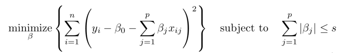
The first equation is ridge and the second is lasso…
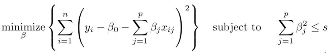
When we fit penalized regression model, we are identifying coefficients that minimize RSS. However, we must accomplish this while being constrained by a budget s. This budget determines how large |βj| (in the case of lasso) and βj2 (in the case of ridge) can be.
Contours of the error and constraint functions:
Take a look at the graph below. βˆ (Beta hat) in all three graphs is the OLS solution. The constraint region is represented by a solid shape: the yellow square is for lasso, the blue circle is for ridge, and the beige rectangle with curved edges is for elastic net regression. The constraint region always needs to be smaller than or equal to the budget s.
The ellipses represent contours of the error. If the penalty is small (e.g. no penalty or λ=0), the constraint regions will include βˆ.

Contours of the error and constraint functions: Constraint is the sum of absolute squares, and the green ellipses are the contours of RSS. The red dot is the smallest RSS that meets the budget s (solution).
The ellipses that are centered around βˆ represent regions of constant RSS, and values on a single ellipse have the same value as RSS. As we move farther away from the OLS coefficient estimates, RSS increases.
Coefficient estimates for lasso, ridge and elastic net regressions are represented by red points where the ellipse touches the constraint region. When the constraint region is a square, the ellipse will touch it at an axis. In contrast, a constraint region that is a circle will typically not touch the ellipse at an axis (and none of the coefficients will be zero). Elastic net is a hybrid of lasso and ridge and its ellipses will not touch the constraint region at the axis but it may come very close.
So then why not use one of the three models all the time? The accuracy of one model based on test data is not guaranteed to surpass the test accuracy of the other model. The shrinkage of three models differs greatly: In ridge regression, the coefficients are reduced by the same proportion, while in lasso regression, the coefficients are shrunken towards zero by a constant amount (λ/2). Any coefficient that is less than λ/2 is reduced to zero. Elastic net will be somewhere in between.
