Dimension Reduction: Principal Components and Partial Least Squares Regression

““Man’s mind once stretched by a new idea, never regains its original dimension.””

— Oliver Wendell Holmes

Objectives:

• Explain how principal components regression and partial squares regression work.

• Show Python code to to perform Principal Components Regression and Partial Least Squares Regression

Overview:

Principal Components Regression (PCR) and Partial Least Squares Regression (PLS) are yet two other alternatives to simple linear model fitting that often produces a model with better fit and higher accuracy. Both are dimension reduction methods but PCR offers an unsupervised approach, while PCL is a supervised alternative.

Principal Components Regression:

The approach is based on reducing the number of predictors into a smaller dimension using principal components analysis.  These principal components then are used as regressors when fitting a new OLS model. 

Since a relatively small number of principal components explain a large percent of the variability in data, the approach may be sufficient in explaining a relationship between the target variable and the principal components that were constructed from a larger number of regressor variables.

One drawback of PCR, is that it is based on an unsupervised approach to feature reduction: Principal Components Analysis. PCA is set out to find linear combinations that best describe original regressors. Since detection of these linear combinations was performed without using a target variable, we can’t be certain that the principal components we created are the best to use to predict the target variable. It is entirely possible, that a different set of principal components would perform better. The solution to this problem is Partial Least Squares Regression (more about that later).

Still, the PCA approach is a good way to overcome multicollinearity problems in OLS models.  Further, since PCA is a dimension reduction approach, PCR may be a good way of attacking problems with high-dimensional covariates. 

 PCR follows three steps:

1.     Find principal components from the data matrix of original regressors.

2.     Regress the outcome variable on the selected principal components, which are covariates of the original regressors.  The regression used should be OLS.

3.     Transform the findings back to the scale of the covariates using PCA loadings to get a PCR estimator so that regression coefficients can be estimated.    

 PCR vs. Shrinkage:

Sometimes, PCR can outperform shrinkage models (in terms of model error), while other times shrinkage models are better.  If relatively few principal components are needed to explain variance in the data, then PCR will outperform shrinkage methods such as ridge, lasso or elastic net models.  If more principal components are required, then shrinkage methods will perform better. 

Principal Components Regression and the Boston Housing Data:

First, we need load all required libraries, most of them as part of the sklearn package

import pandas as pd
import statsmodels.api as sm
import numpy as np
import sklearn

%matplotlib inline

import pandas as pd
import numpy as np
import matplotlib.pyplot as plt

from sklearn.preprocessing import scale 
from sklearn import model_selection
from sklearn.decomposition import PCA
from sklearn.linear_model import LinearRegression
from sklearn.metrics import mean_squared_error
from sklearn.preprocessing import StandardScaler
from sklearn.preprocessing import PolynomialFeatures
from sklearn.cross_decomposition import PLSRegression, PLSSVD

Process the data, by transforming all variables using box-cox transformation.

#load and partition data
from sklearn.datasets import load_boston
boston= load_boston()

boston_features_df = pd.DataFrame(data=boston.data,columns=boston.feature_names)
boston_target_df = pd.DataFrame(data=boston.target,columns=['MEDV'])

#Transform data 
#add one to each value to get rid of 0 values in both target and features

numeric_cols = [col for col in boston_features_df if boston_features_df[col].dtype.kind != 'O']
numeric_cols
numeric_cols2 = [col for col in boston_target_df if boston_target_df[col].dtype.kind != 'O']
numeric_cols2

boston_features_df[numeric_cols] += 1
boston_target_df[numeric_cols2] += 1
boston_features_df.head()
boston_target_df.head()

#Box-Cox Transform features
column_trans = ColumnTransformer(
    [('CRIM_bc', PowerTransformer(method='box-cox', standardize=True), ['CRIM']),
     ('ZN_bc', PowerTransformer(method='box-cox', standardize=True), ['ZN']),
     ('INDUS_bc', PowerTransformer(method='box-cox', standardize=True), ['INDUS']),
     ('CHAS_bc', PowerTransformer(method='box-cox', standardize=True), ['CHAS']),
     ('NOX_bc', PowerTransformer(method='box-cox', standardize=True), ['NOX']),
     ('RM_bc', PowerTransformer(method='box-cox', standardize=True), ['RM']),
     ('AGE_bc', PowerTransformer(method='box-cox', standardize=True), ['AGE']),
     ('DIS_bc', PowerTransformer(method='box-cox', standardize=True), ['DIS']),
     ('RAD_bc', PowerTransformer(method='box-cox', standardize=True), ['RAD']),
     ('TAX_bc', PowerTransformer(method='box-cox', standardize=True), ['TAX']),
     ('PTRATIO_bc', PowerTransformer(method='box-cox', standardize=True), ['PTRATIO']),
     ('B_bc', PowerTransformer(method='box-cox', standardize=True), ['B']),
     ('LSTAT_bc', PowerTransformer(method='box-cox', standardize=True), ['LSTAT']),
    ])

transformed_boxcox = column_trans.fit_transform(boston_features_df)
new_cols = ['CRIM_bc', 'ZN_bc', 'INDUS_bc', 'CHAS_bc', 'NOX_bc', 'RM_bc', 'AGE_bc', 'DIS_bc','RAD_bc','TAX_bc','PTRATIO_bc', 'B_bc', 'LSTAT_bc']

boston_features_bc = pd.DataFrame(transformed_boxcox, columns=new_cols)
pd.concat([ boston_features_bc], axis = 1)
boston_features_bc.head()
##### Box-Cox tranform target
column_trans = ColumnTransformer(
    [('MEDV_bc', PowerTransformer(method='box-cox', standardize=True), ['MEDV']),
    ])
transformed_boxcox = column_trans.fit_transform(boston_target_df)
new_cols2 = ['MEDV_bc']

boston_target_bc = pd.DataFrame(transformed_boxcox, columns=new_cols2)
pd.concat([ boston_target_bc], axis = 1)
boston_target_bc.head()

Partition the data and create polynomial features and interaction terms. Also select a few variables from a larger dataset (p=29).

#Partition the data based on box-cox transformed dataframes 
X = boston_features_bc
Y = boston_target_bc
X_train, X_test, Y_train, Y_test = sklearn.model_selection.train_test_split(X, Y, test_size = 0.20, random_state = 5)
X_train.head(3)
# Create interaction terms (interaction of each regressor pair + polynomial)
#Interaction terms need to be created in both the test and train datasets
interaction = PolynomialFeatures(degree=2, include_bias=False, interaction_only=False)

#X traning
#Note the use of input_features=boston.feature_names which switches back to nomenclature without _bc
X_interact_train = pd.DataFrame(interaction.fit_transform(X_train), columns=interaction.get_feature_names(input_features=boston.feature_names))
print(X_interact_train.head(3))

#X test
#Note the use of input_features=boston.feature_names which switches back to nomenclature without _bc
X_interact_test = pd.DataFrame(interaction.fit_transform(X_test), columns=interaction.get_feature_names(input_features=boston.feature_names))

#Since X_inter is used in regression, the index of the that dataset and the outcome variable must be the same
#Reset the index of Y manually 
#Y training
Y_interact_train=Y_train.reset_index()
Y_interact_train=Y_interact_train.drop(['index'], axis=1)

#Y test
Y_interact_test=Y_test.reset_index()
Y_interact_test=Y_interact_test.drop(['index'], axis=1)
print(Y_interact_test.head(3))

#Select columns with approprite interactions from prior analysis
selected_train_X=X_interact_train[['CRIM', 'ZN', 'INDUS', 'CHAS', 'NOX', 'RM', 'AGE', 'DIS', 'TAX', 'RAD', 'PTRATIO', 'B','LSTAT', 'RM^2', 'RM LSTAT', 'RM TAX', 'RM RAD', 'RM PTRATIO', 'LSTAT^2', 'INDUS RM', 'NOX RM', 'RM AGE', 'RM DIS', 'ZN RM', 'CRIM RM', 'RM B', 'DIS^2', 'CRIM CHAS', 'INDUS DIS']]
selected_test_X=X_interact_test[['CRIM', 'ZN', 'INDUS', 'CHAS', 'NOX', 'RM', 'AGE', 'DIS', 'TAX', 'RAD', 'PTRATIO', 'B','LSTAT', 'RM^2', 'RM LSTAT', 'RM TAX', 'RM RAD', 'RM PTRATIO', 'LSTAT^2', 'INDUS RM', 'NOX RM', 'RM AGE', 'RM DIS', 'ZN RM', 'CRIM RM', 'RM B', 'DIS^2', 'CRIM CHAS', 'INDUS DIS']]

Sklearn does not have a PCR module, so we need to run PCA first, and then use the principal components in OLS regression.

#Run principal component analysis
#Scale traning data 
pca = PCA()
X_PCA_train = pca.fit_transform(scale(selected_train_X))

#print a few principal components to check
pd.DataFrame(pca.components_.T).loc[:5,:5]

Note that I only included 29 variables, therefore the maximum number of principal components is 29, e.g. when every variable is considered a principal component. Obviously we need to cut this number down a bit, but for now, I wanted print the first five:

	0	1	2	3	4	5
0	-0.008199	0.345251	-0.025494	0.141112	-0.161930	-0.042164
1	0.102166	-0.248773	-0.207277	0.093519	-0.227399	-0.070631
2	-0.075600	0.328000	-0.007681	0.020806	0.091773	0.012903
3	-0.005331	0.016206	0.021662	0.265715	0.378872	0.346467
4	-0.042239	0.338981	0.093822	0.110351	0.085338	0.053289
5	-0.017848	-0.184281	0.154052	0.461135	-0.187616	-0.098466

Next we will run cross validation to calculate the MSE value of each model as we place more and more principal components in linear regression.

n = len( X_PCA_train)
print(n)

#Run 10-fold cross-validation and compute MSE:
ten_fold = model_selection.KFold( n_splits=10, shuffle=True, random_state=1)

#regression function from sklearn and empty list for mse
regr = LinearRegression()
mse = []

# First, calculate MSE with intercept only
MSE_value = -1*model_selection.cross_val_score(regr, np.ones((n,1)), Y_interact_train['MEDV_bc'].ravel(), cv=ten_fold, scoring='neg_mean_squared_error').mean()    
mse.append(MSE_value)

#The maximum number of principal componens is 29 where each variable is a principal component
# Calculate MSE using CV for each of the 29 principle components
#Add PCs one by one
for i in np.arange(1, 30):
    MSE_value = -1*model_selection.cross_val_score(regr, X_PCA_train[:,:i], Y_interact_train['MEDV_bc'].ravel(), cv=ten_fold, scoring='neg_mean_squared_error').mean()
    mse.append(MSE_value)
    
# Plot results    
plt.plot(mse, '-v')
plt.xlabel('No. of PC in Regression')
plt.ylabel('MSE')
plt.title('Model MSE as No. of Principal Components Change')
plt.xlim(xmin=-1);

The graph below shows that the MSE decreases rapidly and significantly as the first few principal components are used but it tails off and provides very little improvement after about the 6th principal component. Further, the MSE remains close to unchanged after 10 or more principal components are included in the model.

We can also calculate and plot the aggregate variance explained as we put more and more principal components in the model. The first principal component explains 27% of the variance but adding the first seven means that 85% of the variance is captured, meaning we do not need to go beyond this number to explain the model very well.

pct_var_rate=np.cumsum(np.round(pca.explained_variance_ratio_, decimals=4)*100)
pct_var_rate

array([26.86, 50.56, 57.9 , 64.45, 69.14, 73.06, 76.45, 79.31, 82.02,
       84.66, 86.67, 88.67, 90.45, 91.9 , 93.19, 94.21, 95.11, 95.91,
       96.51, 97.07, 97.58, 98.02, 98.41, 98.78, 99.09, 99.39, 99.63,
       99.85, 99.99])

import matplotlib.pyplot as plt
plt.plot(pct_var_rate)
plt.ylabel('Percent')
plt.title('Pct of Variance Explained as No. of Principal Components Change')
plt.show()

Now we can fit an OLS model with only the selected number of principal components and calculate the models MSE on test data. The test MSE was 0.32109279891577586. The test MSE of ridge regression on the same data was 0.20453122412502994 (See the post on regularized regression), therefore PCR did not get us a model that is better than ridge regression this time. This is not surprising, because the number of principal components was relatively large, which usually favors ridge regression.

X_PCA_test = pca.transform(scale(selected_test_X))[:,:4]

# Train regression model on training data 
regr = LinearRegression()
regr.fit(X_PCA_train[:,:4], Y_interact_train)

# Prediction with test data
pred = regr.predict(X_PCA_test)
mean_squared_error(Y_interact_test, pred)

Partial Least Squares:

PLS is also a feature reduction method but it offers a supervised alternative to PCR. The new set of features are also the linear combinations of the original regressors, but in computing them, the method makes use of the target variable. As a result, the results of this technique not only explain the linear combinations of original features but the response variable as well.

The model first requires the standardization of all predictors. PLS then starts computing the first linear combination of features by setting constants used in computing the Z values (Z values represent the linear combinations of original predictors) equal to the coefficient of simple OLS regression between the target and a specific regressor. PLS puts more weight on variables that are more correlated with the target variable.

#Partial Least Squares

# 10-fold CV, with shuffle
ten_fold = model_selection.KFold(n_splits=10, shuffle=True, random_state=1)

mse = []

for i in np.arange(1, 30):
    pls = PLSRegression(n_components=i)
    score = model_selection.cross_val_score(pls, scale(selected_train_X), Y_interact_train['MEDV_bc'], cv=ten_fold, scoring='neg_mean_squared_error').mean()
    mse.append(-score)
# Plot results
plt.plot(np.arange(1, 30), np.array(mse), '-v')
plt.xlabel('No. of PLS Components in Regression')
plt.ylabel('MSE')
plt.title('Model MSE as No. of PLS Components Change')
plt.xlim(xmin=-1)

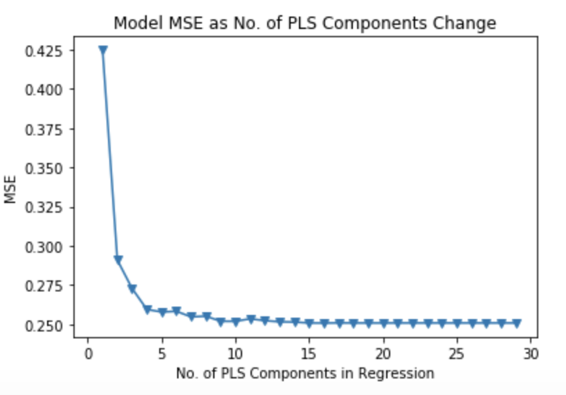
Now we are ready to compute the test MSE achieved by the model. Here, we are introducing only the first six components because the test MSE is minimized at that level. The test MSE of this model is significantly better than that of PCR at 0.20540507220365029. In fact, it is only slightly worse than that of ridge regression (0.20453122412502994).

# Train regression model on training data 
pls = PLSRegression(n_components=6)
pls.fit(scale(selected_train_X), Y_interact_train)

# Prediction with test data
pred2 = pls.predict(selected_test_X)
mean_squared_error(Y_interact_test, pred2)