Multinomial Logistic Regression

““You can lead a horse to water but you can’t make him enter regional distribution codes in data field 97 to facilitate regression analysis on the back end. “”

— John Cleese

OBJECTIVES:

This blog focuses solely on multinomial logistic regression. Discussion about binary models can be found by clicking below:

• binary logit

• binary probit and complementary log-log

The discussion below is focused on fitting multinomial logistic regression models with sklearn and statsmodels.

• Get introduced to the multinomial logistic regression model;

• Understand the meaning of regression coefficients in both sklearn and statsmodels;

• Assess the accuracy of a multinomial logistic regression model.

Introduction:

At times, we need to classify a dependent variable that has more than two classes.  For this purpose, the binary logistic regression model offers multinomial extensions.  Multinomial logistic regression analysis has lots of aliases: polytomous LR, multiclass LR, softmax regression, multinomial logit, and others. Despite the numerous names, the method remains relatively unpopular because it is difficult to interpret and it tends to be inferior to other models when accuracy is the ultimate goal.

Multinomial Logit:

Multinomial logit models represent an appropriate option when the dependent variable is categorical but not ordinal.  They are called multinomial because the distribution of the dependent variable follows a multinomial distribution.

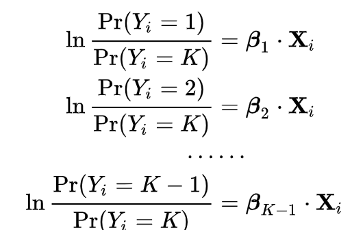
When fitting a multinomial logistic regression model, the outcome has several (more than two or K) outcomes, which means that we can think of the problem as fitting K-1 independent binary logit models, where one of the possible outcomes is defined as a pivot, and the K-1 outcomes are regressed vs. the pivot outcome.

Exponentiating both sides of the equations will provide probabilities:

The multinomial logit model uses maximum likelihood estimation.  The first iteration is a model with no regressors, only the intercept.  The next iteration includes regressors in the model. The regressors are changed at every iteration, and iterations continue until the model is said to have converged.   The log likelihood decreases until a model converges, e.g. the next iteration would not produce a lower log likelihood.  See

Using Sci-Kit Learn:

In order to demonstrate how to use Sci-Kit Learn for fitting multinomial logistic regression models, I used a dataset from the UCI library called Abalone Data Set. While most projects try to identify the age of abalone based on several features, I tried to classify abalone instead to show the how LogisticRegression works :

• Category 1: Male (n= 1,516)

• Category 2: Infant  (n=1,324)

• Category 3: Female (n=1,301)

#load all necessary libraries
import pandas as pd 
import numpy as np 
import scipy as scp
import sklearn

from sklearn.model_selection import train_test_split
from sklearn.linear_model import LogisticRegression
from sklearn.metrics import classification_report
from sklearn import metrics 
from sklearn.metrics import confusion_matrix

#read the dataset
#note that the csv file is space delimited
abalone_df = pd.read_csv('abalone-3.csv',  delimiter=' ') 
abalone_df.head()

import statsmodels.api as sm
import matplotlib.pyplot as plt

There are 10 variables of which the first - SEX - will be used as the dependent variable. Also, CLASS is formatted as string and needs to be converted to integer format. For that purpose, I dropped the first character (A), and kept the second character as an integer. I stored this data in a newly created variable called SIZE_CLASS.

Abalone_sex=abalone_df['SEX'].value_counts()
Abalone_class=abalone_df['CLASS'].value_counts()
print(Abalone_sex)
print(Abalone_class)

M    1516
I    1324
F    1301
Name: SEX, dtype: int64
A3    1318
A2     945
A4     747
A1     440
A6     364
A5     327
Name: CLASS, dtype: int64

#Recode CLASS to integer: LinearRegression does not take string
def Classification(CLASS):
    if CLASS == 'A1':
        return 1
    elif CLASS == 'A2':
        return 2
    elif CLASS == 'A3':
        return 3
    elif CLASS == 'A4':
        return 4
    elif CLASS == 'A5':
        return 5
    elif CLASS == 'A6':
        return 6
    
abalone_df['SIZE_CLASS']=abalone_df['CLASS'].apply(Classification)

Description of Data:

The data is sourced from study of Abalone in Tasmania. It can be found at the UCI Machine Learning Repository. The dataset contains 4,141 observations and 10 variables.

1. SEX = M (male), F (female), I (infant)

2. LENGTH = Longest shell length in mm

3. DIAM = Diameter perpendicular to length in mm

4. HEIGHT = Height perpendicular to length and diameter in mm

5. WHOLE = Whole weight of abalone in grams

6. SHUCK = Shucked weight of meat in grams

7. VISCERA = Viscera weight in grams

8. SHELL = Shell weight after drying in grams

9. RINGS = Age (+1.5 gives the age in years)

10. CLASS = Age classification from 1 to 6 (A1= youngest,..., A6=oldest)

We are now ready to partition the dataset:

#Create training and test datasets
#CLASS was recoded into SIZE_CLASS to change from string to integer
#CLASS needs to be dropped
X = abalone_df.drop(['SEX', 'CLASS'], axis=1) 
y = abalone_df['SEX']

print(list(X.columns.values)) 

X_train, X_test, y_train, y_test = sklearn.model_selection.train_test_split(X, y, test_size = 0.20, random_state = 5)
print(X_train.shape)
print(X_test.shape)
print(y_train.shape)
print(y_test.shape)

['LENGTH', 'DIAM', 'HEIGHT', 'WHOLE', 'SHUCK', 'VISCERA', 'SHELL', 'RINGS', 'SIZE_CLASS']
(3312, 9)
(829, 9)
(3312,)
(829,)

Using the training data, we can fit a Multinomial Logistic Regression model, and then deploy the model on the test dataset to predict classification of individual abalone.

model1 = LogisticRegression(random_state=0, multi_class='multinomial', penalty='none', solver='newton-cg').fit(X_train, y_train)
preds = model1.predict(X_test)

#print the tunable parameters (They were not tuned in this example, everything kept as default)
params = model1.get_params()
print(params)

{'C': 1.0, 'class_weight': None, 'dual': False, 'fit_intercept': True, 'intercept_scaling': 1, 'l1_ratio': None, 'max_iter': 100, 'multi_class': 'multinomial', 'n_jobs': None, 'penalty': 'none', 'random_state': 0, 'solver': 'newton-cg', 'tol': 0.0001, 'verbose': 0, 'warm_start': False}

Intercept and Coefficients:

The intercept and coefficients are stored in model1.intercept and model1. coef_ respectively. Here we need to spend a bit of time, because the output of Sci-Kit Learn is different from what we may expect.

#Print model parameters
print('Intercept: \n', model1.intercept_)
print('Coefficients: \n', model1.coef_)

Intercept: 
 [-1.68390042  0.83893379  0.84496662]
Coefficients: 
 [[-5.57907614  6.04845251  3.83162954  2.20508227 -2.72608507  5.10634046
  -2.59338756  0.04532049  0.0479457 ]
 [11.50479079 -6.39406857 -5.06935755 -3.82813431  2.15067035 -8.50130706
   3.80799702 -0.06045528 -0.15593219]
 [-5.92571465  0.34561606  1.23772801  1.62305204  0.57541472  3.3949666
  -1.21460946  0.01513479  0.10798649]]

The first array contains three intercepts and the second array contains three sets of regression coefficients.  This is different from what we may be used to in SAS and R.  In fact, the sklearn based output is different from the statsmodel version (A discussion of Multinomial Logistic Regression with statsmodels is available below). Let’s see why…

In this solution, there is an equation for each class. These act as independent binary logistic regression models. The actual output is log(p(y=c)/1 - p(y=c)), which are multinomial logit coefficients, hence the three equations.  After exponentiating each regressor coefficient, we in fact get odds ratios. The interpretation of the coefficients is for a single unit change in the predictor variable, the log of odds will change by a factor indicated by the beta coefficient, given that all other variables are held constant. Log of odds is not really meaningful, so exponentiating the output gets a slightly more user friendly output:

#Calculate odds ratio estimates
import numpy as np
np.exp(model1.coef_)

array([[3.77605244e-03, 4.23457228e+02, 4.61376600e+01, 9.07099784e+00,
        6.54751188e-02, 1.65065185e+02, 7.47663353e-02, 1.04636316e+00,
        1.04911369e+00],
       [9.91898326e+04, 1.67144197e-03, 6.28645758e-03, 2.17501568e-02,
        8.59061520e+00, 2.03202598e-04, 4.50600939e+01, 9.41335866e-01,
        8.55617206e-01],
       [2.66989896e-03, 1.41286005e+00, 3.44777127e+00, 5.06853610e+00,
        1.77786770e+00, 2.98136577e+01, 2.96825914e-01, 1.01524990e+00,
        1.11403269e+00]])

The interpretation of the exponentiated coefficients is for a single unit change in the predictor variable, the odds will be multiplied by a factor indicated by the exponent of the beta coefficient, given that all other variables are held constant. For example, the first variable is LENGTH with a value of 0.038. This means that if length increases by one unit the odds of being female is 3.8% compared to the status when length did not increase by one unit. A generic output looks looks something like this (the below is based on infants!)

Statsmodels:

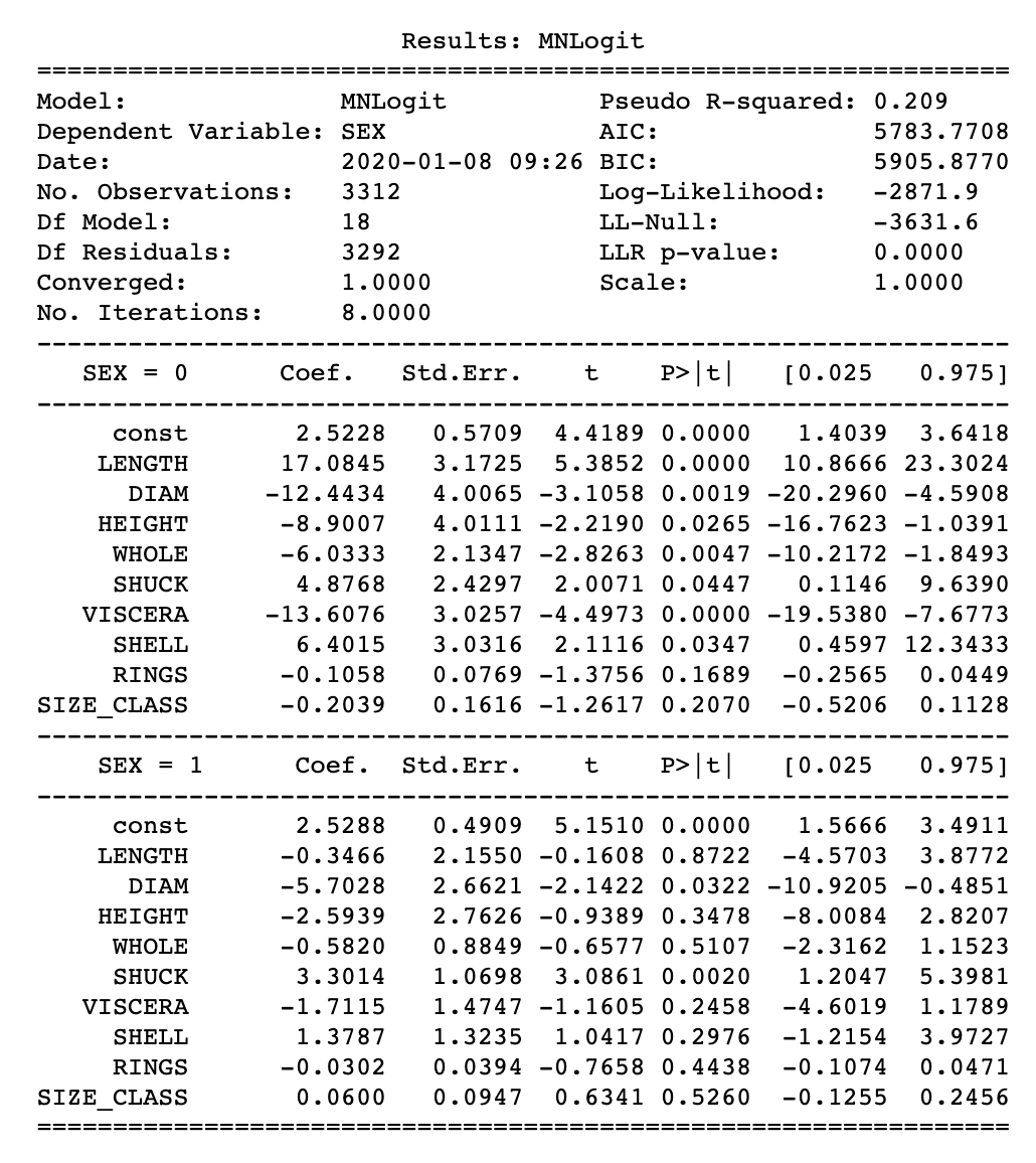
Notice that the statsmodels output is very different from that of sklearn. In this case, there are K-1, in this case two equations, which show coefficients against a reference group. In the abalone example, the reference group was chosen to be female. The coefficients represent the log of ratios between two probabilities: the probability of belonging to a group of interest vs. the probability of belonging to the reference group. In the abalone example, the reference group was female, therefore the equation below represents the first set of coefficients marked as SEX=Infant. Note that there are two sets of coefficients, one marked as Infant and the second marked as Male.

#Use statsmodels to assess variables

logit_model=sm.MNLogit(y_train,sm.add_constant(X_train))
logit_model
result=logit_model.fit()
stats1=result.summary()
stats2=result.summary2()
print(stats1)
print(stats2)

So how do we interpret this data? For example, the coefficient LENGTH is 17.1 for the Infant group.  This means that increasing the LENGTH measurement by one unit will result in an increase by 17.1 units in the log of the ratio between the probability of being an infant vs. the probability of being female. Very complicated…but that doesn’t matter if the goal is to accurately predict an outcome.

Accuracy:

Assessing the accuracy of the model is not difficult but errors at the different levels act as a compounding problem.

#Create a confusion matrix
#y_test as first argument and the preds as second argument 
confusion_matrix(y_test, preds)

array([[ 88,  34, 135],
       [ 11, 223,  28],
       [ 88,  63, 159]])

#transform confusion matrix into array
#the matrix is stored in a vaiable called confmtrx
confmtrx = np.array(confusion_matrix(y_test, preds))
#Create DataFrame from confmtrx array 
#rows for test: Male, Female, Infant designation as index 
#columns for preds: male, predicted_female, predicted_infant as column

pd.DataFrame(confmtrx, index=['Female','Infant', 'Male'],
columns=['predicted_Female', 'predicted_Infant', 'predicted_Male'])

#Accuracy statistics

print('Accuracy Score:', metrics.accuracy_score(y_test, preds))  

#Create classification report
class_report=classification_report(y_test, preds)
print(class_report)

Accuracy Score: 0.5669481302774427
              precision    recall  f1-score   support

           F       0.47      0.34      0.40       257
           I       0.70      0.85      0.77       262
           M       0.49      0.51      0.50       310

    accuracy                           0.57       829
   macro avg       0.55      0.57      0.56       829
weighted avg       0.55      0.57      0.55       829

The accuracy of this model is poor with only 57% of predictions being correct. The precision and recall of female and male abalone is very concerning as well.